Tales of FPGA - Road to SDRAM - E02

Posted on August 16, 2022 in hacks

This post is the second one of a serie which starts with Episode 1, in which we have presented what FPGA are, how to control them, and implicitly discovered their major benefit: they make the physical world rational and clean.

Indeed, the physical world a.k.a. "reality" is notoriously messy, as anyone who has tried to implement some design with discrete electronic components knows.

For instance, should we decide that "zero" is +0V and "one" is +5V... there are chances that the transistor-based AND gate that we carefully assembled on our breadboard outputs +4.8V for "one" and not +5V because, imperfections. If we feed that signal into anoter gate, it will probably be identified as "one". But if we keep doing this, then at one point we will end up with a +2.6V signal and what is that supposed to mean exactly? "Zero", or "one"? Our design lacks additional circuitry to ensure that we maintain the correct signal levels everywhere, we feed enough current, etc.

Another example: these 30 cm of wire flying over our breadboard and carrying a signal at, say, 100MHz? It is an antenna in the FM radio frequencies. It is going to broadcast that signal, as well as be impacted by existing radio signals on that frequency. Our design may randomly fail and, if carefully examining signals with a scope, we would see all sorts of very weird distortions.

FPGA have none of this: they are clean and reproducible. We write text files, have them processed by a tool, and end up with a hardware-level design that just works. If we make a mistake, there is no need for rewiring things, going to the shop to buy that one component we are missing, etc. We do not have to worry about radio interferences, current leaks, etc.

With FPGA, the physical world becomes deterministic.

Meet the Enemy

And yet, the FPGA designer has one enemy, and this enemy is time.

It is convenient to think of a LUT2 as something that immediately updates its output according to its inputs. In reality, it is almost immediate. In the FPGA chip we are using (a Xilinx Spartan-7 family chip), the delay would be around .15ns or 150ps. A flip-flop has a delay of about .55ns or 550ps.

Sure, 150ps is 0.000 000 000 150s and this is very small. Yet, the period of a 4GHz signal—a value one can meet in modern CPUs—is 250ps: a very small value too, but one which is very comparable, in scale, to the above delay.

It is also convenient to think of connections betweens elements as pure electric wires, carrying signals at the speed of light. In reality, signals travels the FPGA die at a slower speed, because connections are not just true electric wires. And then even at the speed of light, electricity only travels about 30cm per ns, or 3mm in 10ps, and considering the size of a typical chip die, 3mm might be the distance separating two LUTs.

Let us see what this means with an example.

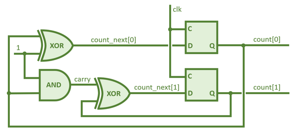
This circuit increments a two-bits signal on every clock tick. The new square boxes are flip-flops: they update their output (the Q port) to reflect the value of their input (the D port) on each raising edge of their clock (the C port). So count will go 00, 01, 10, 11, 00, 01, etc. each time the clock ticks.

More precisely, when the clock ticks,

• Flip-flops update their output to match their input after about .55ns
• Gates update their output to match their inputs after about .15ns

So, count_next[1] will reach its new value after .55 + .15 + .15 = .85ns. This is called the propagation delay. And still, we cannot tick the clock immediately, because the flip-flops demand that the input be stable for some amount of time before the clock ticks: this is call the setup time. It is about .05ns in our case. And thus, the clock can only ticks again after .9ns have elapsed.

We are ignoring the connection delays here. So, let's round it all to 1ns. This corresponds to a frequency of 1GHz. Not too bad, but this is a very simple circuit.

Very quickly, things get complex, and the maximum frequency can fall down to 100MHz or even 10MHz. If we do not respect that constraint, things become completely unpredictable. If we are only slightly too fast, we might not respect the setup time, thus creating a situation called metastability: the data coming out of flip-flops may be randomly wrong. And of course, if we are really too fast, everything becomes random.

Know Thy Enemy

Tools such as the Vivado IDE do not simply convert code into a network of LUTs, flip-flops, etc. They also decide which elements to use on the chip (which can contain a few thousands LUTs, for instance), trying to minimize the physical distance between elements. And then, they process the resulting network and calculate all the propagation times and finaly issue a timing report.

Take the LED blinker from the previous episode. We would tell Vivado that the clock signal comes from "outside" of the chip, actually an oscillator on the development board, which runs at 12MHz. Vivado would report that at 12MHz, everything is fine. There is another oscillator on the board, which runs at 100MHz, and that should be OK too.

But imagine we have a 1GHz clock on the board: Vivado would definitively build the design (which we can then push to the board) but it would also issue timing warnings, telling us that our design has little chance to work.

When that happens, for instance when we try to run our carefully crafted CPU at 10MHz and Vivado complains about timings, there are essentially two solutions:

• Slow the clock. Not very satisfactory, but simple enough
• Refactor the design, maybe doing less per clock cycle (see: pipelining)

Were we not supposed to talk about SDRAMs?

We were, but that little disgression about time will prove useful in the next episode, where we will present the different types of RAM and see how RAM is essentially dictating time constraints in a modern design.

To be continued!